Lecture 13 - Control II

Welcome back to Robot Control. Building directly on Lecture 12, this lecture shifts from basic kinematics and simple feedback loops to the messy reality of robot dynamics and physical interaction.

When you are commanding a complex system—like an anthropomorphic articulated arm—the inertia isn't constant; it changes drastically depending on how the arm is stretched out or folded in. Here is the quickest way to digest the core concepts of Lecture 13 to keep your projects moving.

1. Conquering the Robot's Dynamics

A robot's dynamic model is highly non-linear, dealing with changing inertia matrices $M(q)$, Coriolis/centrifugal forces $C(q,\dot{q})$, and gravity $g(q)$. If you just use simple position control, the arm will struggle under its own weight.

To fix this, the lecture introduces two main approaches:

• Compensating for Gravity: You can add a specific term to your PD controller that constantly calculates and counteracts the exact gravitational pull on the arm at any given pose. The control law becomes $u=g(q)+K_p(q_d-q)-K_d\dot{q}$.

• Inverse Dynamics Control: This is the holy grail of classical control. Instead of just fighting gravity, the controller mathematically cancels out all the non-linear dynamics of the arm so it behaves like a simple, predictable linear system. The resulting control input equation is $u=M(q)[{\ddot{q}}_d+K_d({\dot{q}}_d-\dot{q})+K_p(q_d-q)]+C(q,\dot{q})\dot{q}+g(q)$.

2. Force and Interaction Control

Most tasks require the robot to actually touch the environment (like the classic Peg-in-Hole assembly problem). If a rigid robot expects empty space but hits a slightly misaligned surface, simple position control will ramp up the motor torque until something breaks. To handle interaction safely, we use control schemes that manage the relationship between force and motion:

• Impedance Control: The robot behaves like a virtual mechanical system. When the environment imposes a motion (like pushing the arm), the robot reacts with a computed force. You can program the robot's end-effector to act like a virtual Mass, a Viscous Fluid (damper), or a Spring.

• Admittance Control: This is the inverse. The robot uses a force sensor to measure the force applied by the environment (or a human), and translates that into a resulting motion or position command.

When trying to insert a peg into a hole with tight tolerances, the robot can't just shove it in. It uses these force control principles combined with Spiral Search Patterns (either translating on the plane or rotating) to feel its way into the correct alignment.

3. The Modern Control Landscape

The lecture wraps up by zooming out to show how these classical methods fit into modern robotics:

• Classical Control: Uses the explicit mathematical model of the robot. It is highly stable and interpretable.

• Machine Learning (ML): Relies on data to estimate disturbances or model complex non-linearities that are too hard to calculate manually.

• Reinforcement Learning (RL): An agent learns the control policy through trial-and-error interaction with the environment to maximize a reward, which is great for highly complex, unstructured tasks.

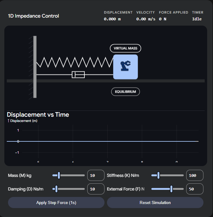
Interactive: Virtual Impedance Controller

To really understand how Impedance Control works on an end-effector, it helps to feel the math. In an impedance control scheme, you dictate how the robot yields to external forces by tuning its virtual mass, damping, and stiffness.

Use the interactive simulator below to apply an external force to a virtual end-effector. Adjust the parameters to see how the robot can be made to act like a stiff spring, a heavy mass, or moving through thick viscous fluid.